This may seem to be a basic topic, but it looks like many people are still confused by the difference between those two concepts. Let us clear this confusion at once!

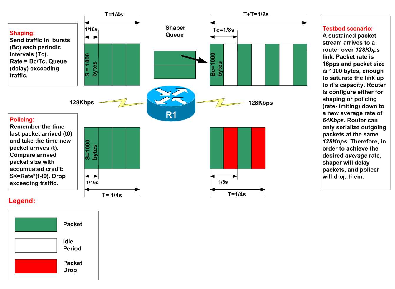
Look at the diagram above. Both router links are clocked at 128Kbps, and the test packet flow has packet size of 1000 bytes each, being sent at a sustained rate of 16 packets per second, effectively saturating the 128Kbps link. Consider what happens when we shape the flow down to 64Kbps. Egress packets are also serialized at 128Kbps - therefore the shaper needs to buffer and delay packets to obtain the target average rate of 64Kbps. Shaper performs that by delaying every burst each Tc interval. For this example, the Bc value (shaper burst) equals to packet size, so effectively every 1/16s interval egress link is busy and the next 1/16s interval it is idle. The average bps rate is total volume of (4*1000) divided by 1/2s (time to send) and multiplied by 8 (to get bps) yielding the result of 64000bps.

The summary points about shaping are as follows:

I) Shaper send Bc amount of data every Tc interval at physical port speed
II) Since shaper delays packets, it uses a queue to store them
III) Shaper queue may use different scheduling algorithms, e.g. WFQ, CBWFQ, FIFO
IV) Shaper unifies traffic flow and introduces delay, which may affect end-to-end QoS characteristics
V) Shaping is generally a WAN technology, used to share a multipoint interface bandwidth and/or compensate for speed differences between sites

On the other hand, policer behaves in a much simpler manner. It achieves the same average traffic rate by dropping a packet that could exceed the policed rate. The policer algorithm is simple: remember the last packet arrival time (“T0”), the current credit (“Cr0”) and “PolicerRate” constant (64Kpbs in our example). (There is also the “Bc” – burst size, but we will ignore it for a moment). When a new packet of size “S” arrives at a moment of time “T” the policer performs the following:

a) Calculate accumulated credit: Cr = Cr0 + (T-T0)*PolicerRate (note: Bc ignored here).
b) If (S <= Cr) than Cr0 = Cr – S and packet is admitted, since we have enough credit
c) Else packet is denied and credit remains the same: Cr0 = Cr.
d) Store the last packet arrival time: T0=T

This simple admission procedure allows for very efficient hardware implementations. Look at the above diagram again. For a sustained packet flow, policer drops every next packet, for it can’t accumulate 1000 bytes of credit during 1/16s (the packet arriving rate) since the “PolicerRate” is just 64000bps. Therefore, every 1/16s the policer is only able to accumulate 500 bytes of credit, and it takes 1/8 of a second to get enough credit to admit a packet.

Now, for the policer burst size. As we remember, with shaping Bc effectively defines the amount of data sent every Tc. With policing it’s purpose is different, however. Look at the diagram below:

The flow no longer sustains. At one moment, the source is paused and then resumed. Policers were designed to take advantage of such irregular behavior. The long pause allows the policer to accumulate more credit and then use it to accept a “large” packet train at once. However, it can’t be allowed for the credit to grow in unbounded manner (e.g. 1 hours of pause between packets yielding very large credit). Therefore, a committed burst size is used by policers as follows:

a) Calculate new credit: Cr = Cr0 + (T-T0)*PolicerRate
b) If (Cr > Bc) then Cr = Bc
c) If (S <= Cr) then Cr0 = Cr – S and packet is admitted.
d) Else packet is denied and Cr0 = Cr.
e) Store the last packet arrival time: T0=T

The Bc constant limits the amount of credit a policer is allowed to accumulate during the idle periods. Obviously, you will never want to set up Bc lower than a network MTU, for this will prohibit any packet from passing admission. Note the following interesting relation: Tc=Bc/PolicerRate. This is sometimes called “averaging interval”. By the policer design, if you observe the policer traffic flow for “Tc” amount of time, you will never see average bitrate to go above “PolicerRate”. Note that policer “Tc” has nothing to do with “shaping” Tc, as they have very different purpose and meaning.

In summary, the key points about policing:

I) Policer uses a simple, credit based admission model
II) Policer never delays packets and never “absorbs” or smoothes packet bursts
III) Policers are usually used at the edge of a network to control packet admission
IV) Policers could be used in either ingress or egress direction

The last question – how would one calculate a Bc value for a policer? As you’ve seen, for a sustained traffic flow it does not matter what size of Bc to pick up – it does not affect the average packet rate. However, in real life, traffic flows are very irregular. If you pick Bc value too small, you may end up dropping too much packets. Obviously, this is bad for protocols like TCP, which consider a dropped packet to be a signal of congestion. Therefore, there exist some general rules of thumb to pick up Bc values based on policer rate. Generally, Bc should be no less than 1,5s*PolicerRate, but you should calculate the optimal value empirically, by running application tests.

Further Reading:
Comparing Traffic Policing and Traffic Shaping for Bandwidth Limiting